Grouping, Sorting, Filtering, Slicers in Pivot Table

Suppose we have the following source data to build our simple Pivot table.

Source Data:

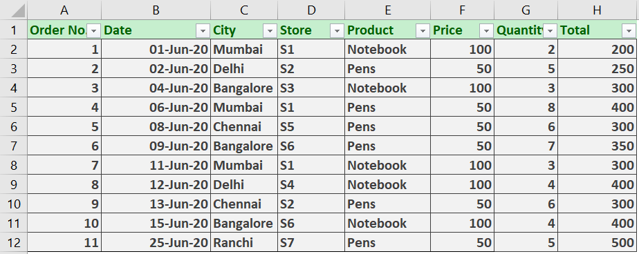
Pivot Table:

Now let us try to Group our data first within the Pivot Table.

Grouping

Let’s first include the field “dates” in our pivot table

To Include a field, click on any cell within the pivot table.

• The pivot table field options appear in the right sidebar of the Excel sheet.

• Select the Desired field to add to the field.

• The fields will now appear in your Pivot Table.

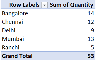
After Including the date field, the quantities are sub-divided into various date row-fields which shows the number of products sold at a particular date in a particular city.

To group this pivot data,

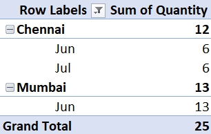
Notice that in our example data all the dates are of the month June. Let’s change some of the months and then group the data.

Group data

1. In the PivotTable, right-click a value and select Group.
2. In the Grouping box, select Starting at and Ending at checkboxes, and edit the values if needed.
3. Under By, select a time period. For numerical fields, enter a number that specifies the interval for each group.
4. Select OK.

Here, we have selected to group our data according to months and set the starting and ending dates as shown below:

And then click on OK

Now we will have our pivot data grouped:

In this way you can group according to the way you want for your data set to be grouped according to your specific work needs.

Filtering in Pivot Table

Excel automatically adds a drop-down filter menu button to the fields when you create a Pivot Table. These filters can help you to get rid of irrelevant data while analyzing and can be used to only view a subset of the data.

Filtering data in a pivot table is as simple as filtering a regular table. Just follow the steps mentioned below:

1. Click on the Filter button beside the column name.
2. Uncheck the Select all option

And select only those values which you want to display.

3. Then Click on OK

You’ll now observe that your pivot table only displays the filtered data and hides the other data.

Only the cities which we selected during the filtering process are present here.

Sorting Data inside Pivot Table

Generally, pivot tables are sorted in the order their source data is sorted. But if you want to change the default sorting behavior of pivot tables. You can do so by following the simple steps mentioned below:

First, we will change the filtering to show all the data. And remove the grouping by date and also remove the date field to show only the quantities.

Our Pivot Table now looks like this:

Now suppose, we want to sort this data in ascending order of their quantities.

Steps:

1. Click on the Filter button beside the column name.
2. Click on More Sort Options

If your sorting jog gets done with the above two options, you can use them also. For now, we will use More sort options to have more options for sorting.

3. A dialog box “Sort” appears,

We want to sort by ascending, so click on the Ascending (A to Z) radio button.

And in the drop-down list we will be selecting according to Sum of Quantity to sort the data based on the no. of quantity of products sold in each city.

Then click on OK.

Now we have our sorted pivot table:

I think it was fairly easy to do all of the above operations.

Off course, your data will be different, but by now you must have got the hang of it. So that you can implement these operations on your own worksheet.

The last topic which we are going to discuss today is How to insert slicers in Pivot tables.

Insert a Slicer

Slicers are interactive elements of a pivot table added after Excel 2010. Slicers are like interactive buttons that allow the user to see what has been chosen in the pivot table.

Steps to insert a slicer:

1. Click anywhere inside your Pivot Table
2. Go to the Pivot Table tools tab on the Ribbon and Click on Analyze
3. Click on Insert Slicer under the Filter category

4. Select the desired fields to insert the slicers

We have selected Product and Store as our slicers

Yay! You now have these slicers inserted:

Now you can click on the data elements inside these slicers to show you the relevant information

That’s all for this tutorial. See you in the next one. Till then,

Keep Learning!