
GETPIVOTDATA function helps users to extract values from a Pivot Table. You can use the GETPIVOTDATA function to prepare reports and dashboards based on Pivot Data.
Syntax:
= GETPIVOTDATA(data_field, pivot_table, [field1, item1, field2, item2], …)
Arguments:
- Data_field: The name of the PivotTable field that contains the data that you want to retrieve. This needs to be in quotes.
- Pivot_table: A reference to any cell, range of cells, or named range of cells in a PivotTable. This information is used to determine which PivotTable contains the data that you want to retrieve.
- [field1, item1, field2, item2]: This is an optional argument. 1 to 126 pairs of field names and item names that describe the data that you want to retrieve. The pairs can be in any order. Field names and names for items other than dates and numbers need to be enclosed in quotation marks.
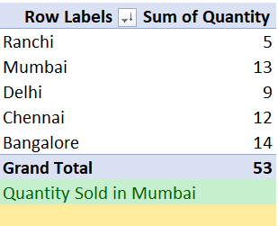
Let us see an example illustrating the working of GETPIVOTDATA function. Suppose we have the following Pivot Table:

Now we want to extract the value of the Quantity of products sold in Mumbai City.
For that we will write the below function:
=GETPIVOTDATA(“Quantity”,$J$2,”City”,”Mumbai”)
The first argument “Quantity” is the name of the field of the Pivot Table from which we want to extract the data.
The Second argument is the reference to the Pivot Table in use.
The Third argument “City” is the Field name which contains the names of the cities in our source data and “Mumbai” is one of the items of the City field from which we want to extract the value corresponding to Mumbai’s quantity field value.
Output of the function:

Also, there is a very easy way to implement this function without writing the formula on your own.
Easy way to use GETPIVOTDATA function
To implement the GETPIVOTDATA function without writing the formula for it is as easy as directly clicking the cell inside the pivot table. We are not joking, its literally possible.
Starting with the Pivot table as it was:
Now just click on the cell you want to extract the data.
Type “=” and then click on the quantity cell corresponding to any item.

You’ll notice Excel automatically fills the exact same formula which gives the exact same output as before.

Well, there is a problem you might face when you decide to hide the field related to the extracted data.
Let us Hide the quantity field from our Pivot Table:

Excel now throws a Reference Error. It is caused due to the fact that you can not display data which is not being actively shown inside a Pivot Table.
Show always remembers this fact that in order to retrieve a Pivot data, the data must be in view. If not, Excel will throw #REF Error.
Thanks for Reading!