Customizing the Layout of Pivot Table in Excel

Pivot table helps the user to expand, isolate, sum, and group the particular data in real time. It can show you the differences in very big data sets and helps in organization of large amounts of data in Excel

Excel mainly provides three defined types of Pivot table layouts to choose from:

1. Compact Form
2. Outline Form
3. Tabular Form

First to create a layout of your choice, you need to create a pivot table (if not created)

Steps to create a Pivot Table:

• Select any Cell from the table you want to create the Pivot Table

We have the above data set with us for this example.

• Go to Insert Tab -> Click on Pivot Table

• A dialog box, Create Pivot Table appears:

Here Select the table/range by first clicking inside the Table/Range field and dragging and selecting the required range.

Then choose where you want to display the pivot table. Here we have chosen to place the table in existing worksheet to help us analyze more effectively.

And then Click on OK.

• Now the option to choose Pivot Table Field Comes:

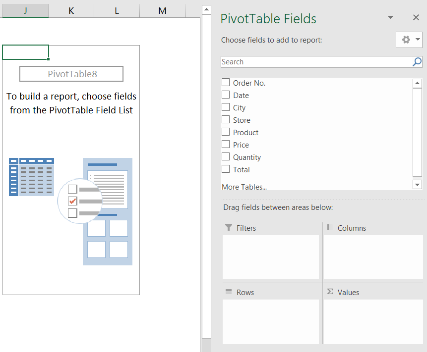
We will choose Date, City and Quantity fields for now.

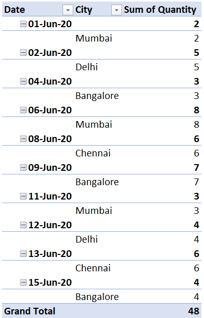
Now that your pivot table has been created it will look something like this:

Here, you can see how effectively we can analyse important information such as on a particular date, we can see the number of quantity of products sold in stores of each city.

This task would be daunting to analyse from the plain tabular database we had.

So, you have the features understood now, let us dive into making reports more fun by defining layouts for pivot tables.

To change the layout:

1. Select any cell in the Pivot Table.

2. Navigate to the Ribbon, under the PivotTable Tools tab -> Click Design tab.

3. On the Layout category -> Click Report Layout

4. Select your desired Report Layout from the options in drop-down menu.

Compact Form

When you choose to have the Report presented in Compact Form, you’ll perceive no change in Pivot Table layout because Compact form is the Default Layout preset for Pivot Tables.

Well, you can clearly notice one thing that the table is condensed quite a bit and the pivot table width is also reduced.

If you are not concerned with field headings and want to quickly analyse the data without much information, Compact form can provide you better productivity.

Compact form displays items from different row area fields in one column and uses indentation to distinguish between the items from different fields. Row labels take up less space in compact form, which leaves more room for numeric data. 

Expand and Collapse buttons are displayed so that you can display or hide details in compact form. Compact form is saves space and makes the PivotTable more readable and is therefore specified as the default layout form for PivotTables.

Tabular Form

Setting Tabular form report layout quickly gives the impression of the increased table width. Now all the fields which we selected have their own fields in the pivot table.

It displays one column per field and provides space for field headers.

It can be useful when you want to show all the fields for better analytics by having reduced the number of rows in the Pivot Table.

Outline Form

Outline Form is similar to tabular form but it can display subtotals at the top of every group because items in the next column are displayed one row below the current item.

Change the way item labels are displayed in a layout form

1. In the PivotTable, select a row field.

This displays the PivotTable Tools tab on the ribbon.

You can also double-click the row field in outline or tabular form, and continue with step 3.

2. On the Analyse or Options tab, in the Active Field group, click Field Settings.

3. In the Field Settings dialog box, click the Layout & Print tab, and then under Layout, do one of the following:
   • To know field items in outline form, click Show item labels in outline form.
   • To display or hide labels from the next field in the same column in compact form, click Show item labels in outline form, and then select Display labels from the next field in the same column (compact form).
   • Find field items in table-like form, click Show item labels in tabular form.

Sources:

https://support.microsoft.com/en-us/office/design-the-layout-and-format-of-a-pivottable-a9600265-95bf-4900-868e-641133c05a80